
Building RAG Systems: A Complete Guide
Imagine asking ChatGPT about your company's refund policy. It either makes something up or tells you it doesn't know. That's not a model problem, that's a data problem. RAG is how you fix that.

1. What is RAG?
RAG stands for Retrieval Augmented Generation. Let’s unpack what that actually means in plain terms.
Think of a regular LLM as a very well-read person who studied everything on the internet up until a certain date, then went into a room with no phone, no books, and no internet. Smart, but limited to what they already know.
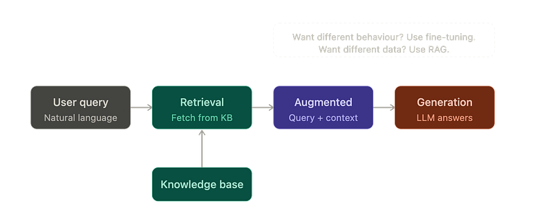
RAG gives that person a library they can look things up in before answering. Here’s how the three parts map to that:
Retrieval is the act of going to the library and fetching the relevant pages. Technically, this means querying a knowledge base, which is where your documents live.
Augmented means the user’s question doesn’t go to the LLM alone. It goes with the retrieved pages attached. The LLM now sees: “Here’s what the user asked, and here’s the relevant context from the knowledge base. Now answer.”
Generation is the final step: the LLM reads everything and produces an answer grounded in your actual data.
Why do we need RAG?
LLMs have two core limitations when it comes to working with your data:
First, they have a knowledge cutoff. Anything that happened after they were trained, they simply don’t know about.
Second, they have a context window limit. You can’t just paste your entire company wiki into a prompt and expect it to work. Even models with large context windows get slower, more expensive, and less accurate as the context grows.
RAG solves both. Instead of stuffing everything into the prompt, you only retrieve what’s relevant to the current question and pass that in. It’s precise, it’s efficient, and it works with documents the model has never seen, your internal policies, product docs, support tickets, anything.
RAG vs fine-tuning
This is the most common question when people first encounter RAG: “Why not just fine-tune the model on my data?”
The distinction comes down to what you’re actually trying to change.
Fine-tuning changes how the model behaves. It’s the right tool when you want the model to adopt a specific tone, follow a certain format, or develop a skill it didn’t have before. For example, training a model to always respond like a customer support agent for your brand.
RAG changes what the model knows. It’s the right tool when the model’s behavior is fine, but it needs access to data it wasn’t trained on. For example, answering questions about a document uploaded by a user five minutes ago.
A useful mental model: fine-tuning is retraining the chef, RAG is handing them a recipe card before they cook.
2. The two pipelines of a RAG system
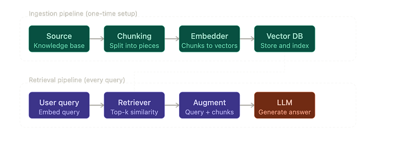
Every RAG system, no matter how simple or complex, is built on two pipelines. Understanding this split is the key to understanding how the whole thing works.
The first is the ingestion pipeline: this is where you prepare your knowledge base and store it in a way that can be searched efficiently. You run this once upfront, and again whenever your data changes.
The second is the retrieval pipeline: this runs every single time a user asks a question. It fetches the relevant context and hands it to the LLM to generate an answer.
A good analogy is a library. Ingestion is the process of acquiring books, cataloguing them, and putting them on shelves in an organized way. Retrieval is what happens when someone walks in and asks a librarian a question. The librarian goes to the right shelf, pulls the relevant pages, and uses them to answer.
3. The ingestion pipeline
The ingestion pipeline is where your raw data gets transformed into something a RAG system can actually search. If this step is done poorly, no amount of clever retrieval logic will save you. Garbage in, garbage out.
It has four steps: source, chunking, embedding, and storing. Let’s go through each.
Step 1: Source (knowledge base)
This is your raw data. It could be a folder of PDFs, a Notion workspace, a database, customer support tickets, product documentation, anything. The knowledge base is everything you want your RAG system to be able to answer questions about.
The important thing to recognize here is that this data hasn’t been processed yet. It’s just raw text in various formats, potentially hundreds of thousands of tokens worth of it. You can’t pass it to an LLM as-is, which is why the next step exists.
Step 2: Chunking
Chunking is the process of splitting your raw text into smaller, manageable pieces. You’re essentially deciding: “How big should each unit of searchable information be?”
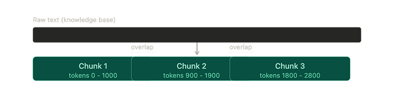
A common default is 1,000 tokens per chunk, but you can tune this up or down depending on your use case.
There’s also a concept called chunk overlap: the last N characters of one chunk are repeated at the start of the next. This exists to prevent a sentence from being cut mid-thought at a chunk boundary, losing its meaning in the process. Think of it like a sliding window moving across your document.
Chunking sounds simple but it’s one of the most consequential decisions in your entire pipeline. Here’s why it can go wrong:
Chunks too small: You preserve precision but lose context. A chunk that says “it increased by 23%” is meaningless without knowing what “it” refers to.
Chunks too large: You retrieve too much noise along with the relevant information, which dilutes the LLM’s answer.
Poor boundaries: Splitting mid-paragraph or mid-table breaks the logical flow of information.
No structural awareness: A naive splitter doesn’t know the difference between a heading, a code block, and body text. It just cuts at character counts, which often produces nonsensical chunks.
This is why there are multiple chunking strategies, and choosing the right one for your document type matters more than most people initially realise.
Now let’s look at the different chunking strategies available and when to use each.
Chunking strategies:
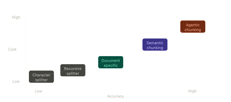
Not all text is structured the same way, so there’s no single chunking strategy that works everywhere. Here are the five main approaches, roughly ordered from simplest to most sophisticated:
Character text splitter is the most basic approach. It splits text at a separator character (a double newline by default), then combines the resulting pieces until they fill up the chunk size limit. If a single piece is already larger than the chunk size, it’s kept as-is. It’s fast and cheap, but completely ignores the meaning of what it’s splitting.
Recursive text splitter is an upgrade on the above. Instead of one separator, you give it a priority list: try splitting by paragraph first, then by sentence, then by word if needed. If a chunk is still too large after the first split, it recursively applies the next separator. This is the default in most RAG frameworks like LangChain for a reason: it respects document structure without being expensive.
Document-specific splitting goes one step further by understanding the file format itself. A PDF splitter knows about pages and columns. A Markdown splitter knows about headers and code blocks. An Excel splitter knows about rows and sheets. Use this when your source documents have rich structure that a generic splitter would destroy.
Semantic chunking is where it gets interesting. Instead of splitting by characters or structure, it splits by meaning. Here’s how it works: every sentence gets encoded into a vector, then sentences are compared against each other using cosine similarity. Sentences above a similarity threshold (commonly the 70th percentile) get grouped into the same chunk. Sentences that diverge in meaning start a new chunk. The result is chunks that are semantically coherent rather than just the right size. The tradeoff is cost: you’re running an embedding model during ingestion, not just doing string operations.
Agentic chunking is the most accurate and the most expensive. You pass the raw text to an LLM with a prompt that says “divide this into logical chunks.” The LLM reads the content with full comprehension and makes chunking decisions the way a human editor would. Reserved for high-stakes use cases where quality matters more than cost.
In practice, production pipelines rarely use any of these in isolation. Libraries like unstructured.io combine multiple strategies under the hood depending on what type of content they’re processing.
Step 3: Embedder
Once your chunks are ready, the next step is to convert each one into a vector, a list of numbers that captures the semantic meaning of that text.
Here’s the intuition: words and phrases that mean similar things end up close to each other in vector space. “Dog” and “puppy” will have vectors that point in nearly the same direction. “Dog” and “quarterly earnings” will not. This is how the retrieval step finds relevant chunks later: it converts the user’s query into a vector and looks for chunks whose vectors are nearby.
The quality of your embedder directly affects the quality of your retrieval. The MTEB leaderboard is the standard benchmark for comparing embedding models. As a reference, OpenAI’s two main options are:
text-embedding-3-small: 1,536 dimensions by default, configurable to 512 or 1,024. Good balance of quality and cost.
text-embedding-3-large: 3,072 dimensions by default. More expressive, captures finer semantic nuance, but more expensive.
More dimensions generally means richer representation, but it also means more storage and slower search. For most applications, text-embedding-3-small is sufficient to start.
Step 4: Vector DB
The final step of ingestion is storing your vectors somewhere they can be searched at query time. This is the vector database.
Choosing the right one mostly comes down to your infrastructure preferences and how far along you are in building:
Pinecone: Fully managed, API-based. Zero infrastructure to maintain. Good choice if you want to move fast and don’t want to think about ops.
Qdrant: Open source and self-hostable. Good if you want control over your data and are comfortable running your own infrastructure.
pgvector: A Postgres extension that adds vector search to your existing database. The best choice if you’re already on Postgres and want to keep your stack simple.
ChromaDB: Extremely easy to set up, runs locally. The go-to for prototyping and experimentation.
FAISS: A Meta library for efficient similarity search. Lightweight, runs in-memory, great for local development or when you need raw speed without a database server.
With step 4 complete, ingestion is done. Your knowledge base is now chunked, embedded, and stored, ready to be searched.
4. The retrieval pipeline
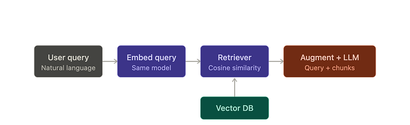
Ingestion was the one-time setup. The retrieval pipeline is what runs live, every single time a user asks a question. It has three steps.
Step 1: Query
The user types a question in natural language. The very first thing the system does is convert that question into a vector, using the exact same embedding model that was used during ingestion.
This point is easy to miss but critical: it has to be the same model. Your chunks were embedded into a specific vector space. Your query needs to land in that same space for similarity search to make sense. Using a different model is like translating a sentence into French to compare it with text in German and expecting the words to align.
Step 2: Retriever
Now that the query is a vector, the retriever takes it and searches the vector DB for the chunks whose vectors are closest to it. The closeness is measured using cosine similarity, which looks at the angle between two vectors:
cosine similarity = (A · B) / (|A| × |B|)
The smaller the angle between two vectors, the more semantically similar the underlying text is. With modern normalized embedding models, the denominator is always 1, so similarity essentially reduces to a dot product between the two vectors.
The retriever returns the top-k most similar chunks. These are the pieces of your knowledge base most likely to contain the answer to the user’s question.
Step 3: LLM generation
The retrieved chunks are combined with the original user query and passed to the LLM as a single prompt. The structure looks something like:
“Here is some context: [chunk 1] [chunk 2] [chunk 3]. Using this context, answer the following question: [user query].”
The LLM now has everything it needs: the question and the relevant information to answer it. This is the augmentation step from our earlier definition, now made concrete. The model generates a response grounded in your actual data rather than just its training weights.
5. History aware retrieval
The three-step retrieval pipeline works well for a single question. But real users don’t ask one question and stop. They have conversations.
Consider this exchange:
User: “What is RAG?”
System: explains RAG
User: “How is it different from fine-tuning?”
That second question, sent to a basic RAG system, is ambiguous. “It” refers to RAG, but the retriever has no idea. It sees the words “different from fine-tuning” and may retrieve completely irrelevant chunks. The conversation history exists in the UI, but the retrieval system is stateless.
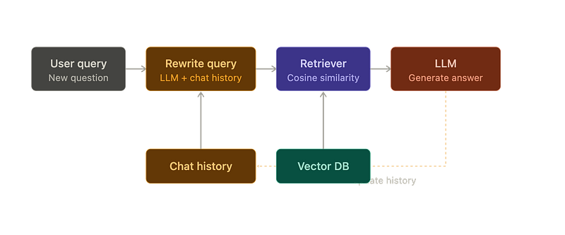
History-aware retrieval solves this by adding a query rewriting step before retrieval. Here’s how it works:
The system stores the full conversation, every question and every answer. When a new question comes in, it doesn’t go straight to the retriever. Instead, the system passes the chat history along with the new question to the LLM and asks it to rewrite the query into a fully self-contained standalone question.
So “How is it different from fine-tuning?” becomes “How is RAG different from fine-tuning?” before it ever reaches the retriever. Now the retrieval is accurate regardless of how many turns deep the conversation is.
Once the answer comes back, the new question and answer are appended to the chat history, and the loop continues.
It adds one LLM call per query, but it’s a small cost for a significant improvement in multi-turn accuracy.
6. Production ingestion pipeline using unstructured.io
Everything we covered in the ingestion pipeline so far was conceptually clean: take your documents, chunk them, embed them, store them. In practice, it’s messier.
Real-world documents are not plain text files. A company’s knowledge base might include PDFs with embedded tables, Word docs with inconsistent formatting, slide decks, spreadsheets, and scanned images. A plain text splitter handed a PDF with a financial table will produce garbage chunks that destroy the meaning of that table entirely.
This is the problem unstructured.io solves. It’s an ETL (extract, transform, load) library built specifically for the chaos of real-world documents. It handles the complexity of mixed content types so your chunking and embedding steps receive clean, structured input. Here’s what a production ingestion pipeline looks like when built with it.
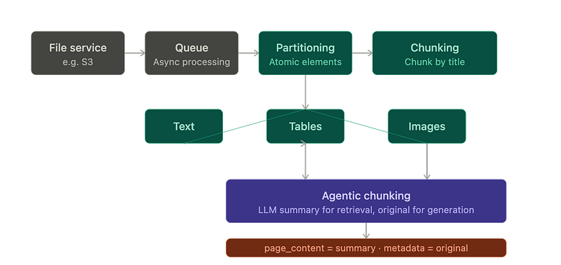
Step 1: File service
Raw documents are uploaded to a file service before any processing begins. S3 is the standard choice here. This gives you a durable, scalable store for source files that’s decoupled from your processing infrastructure, so you can reprocess documents at any time without needing to re-upload them.
Step 2: Queue
Document processing is slow. A large PDF can take several seconds to partition, chunk, and embed. In a production system you never want that blocking a request thread.
Instead, each uploaded file drops a message into a queue. Workers pick up jobs from the queue and process them asynchronously. This keeps ingestion non-blocking and makes the system resilient: if a worker crashes mid-job, the message stays in the queue and gets retried.
Step 3: Partitioning
This is where unstructured.io earns its place. Partitioning is the step that breaks a complex document into its atomic elements: paragraphs of text, tables, images, headers, captions, footers.
This is fundamentally different from chunking. Chunking is about size. Partitioning is about structure. Unstructured reads the document layout first, identifies what type of content each section is, and classifies it before any splitting happens. A table is recognised as a table, not just “some text with a lot of whitespace.” An image is extracted as an image, not skipped.
Step 4: Chunking
Once the document is partitioned into atomic elements, unstructured applies a chunking strategy called “chunk by title.” It keeps all content under the same heading together as a unit, which preserves the semantic relationship between a heading and the paragraphs that follow it.
Images and tables get special treatment here because they can’t just be chunked as text:
Images are stored as base64 encoded data, but the original image file is also retained.
Tables are stored as text chunks, but the original table structure is also retained.
This distinction matters for the next step.
Step 5: Agentic chunking for multimodal chunks
For chunks that contain multimodal content like tables or images, unstructured uses agentic chunking. An LLM is asked to generate a natural language summary of what the chunk contains.
The reason for this split is that retrieval and generation have different requirements. Retrieval needs something compact and semantic, a dense summary that embeds well and surfaces reliably when a user asks a related question. Generation needs the full original content, the actual table with all its rows and values, or the image with all its detail.
So the pipeline stores both, and in LangChain’s document model this maps cleanly to two fields:
page_contentstores the LLM-generated summary, used for embedding and retrievalmetadatastores the original content, passed to the LLM at generation time
The result is a pipeline that retrieves accurately and generates completely, even when your knowledge base is full of charts, tables, and images.
7. Advanced retrieval techniques
Basic retrieval gets you surprisingly far: embed the query, find the most similar chunks, pass them to the LLM. For simple use cases it works fine. But as your knowledge base grows and your users ask more complex questions, the cracks start to show. You get irrelevant chunks, redundant context, and queries that miss relevant information simply because of how they were phrased.
Here are four techniques that meaningfully improve retrieval accuracy in production.
Scored retrieval
The simplest upgrade and the one you should add first.
By default, a retriever returns the top-k chunks regardless of how similar they actually are. If a user asks about your refund policy and your knowledge base doesn’t contain anything about it, basic retrieval will still return the top-k chunks, they’ll just be loosely related noise. The LLM then tries to answer using that noise and either hallucinates or produces a vague, hedged response.
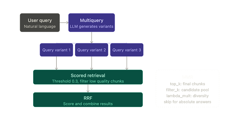
Scored retrieval adds a minimum similarity threshold. Any chunk that scores below it gets dropped, even if it was technically in the top-k. The most common threshold is 0.3. It’s a small change that prevents low-quality context from polluting the prompt and nudging the LLM toward bad answers.
MMR : Max Marginal Relevance
Scored retrieval filters out irrelevant chunks. MMR solves a different problem: redundancy.
Imagine asking “What are the benefits of RAG?” and your top-5 retrieved chunks are all slight variations of the same paragraph from five different pages of the same document. They’re all relevant, but they’re all saying the same thing. You’ve wasted most of your context window passing duplicate information to the LLM.
MMR balances relevance with diversity. It retrieves a larger candidate set first, then selects the final chunks by iteratively picking the one that is both relevant to the query and maximally different from what’s already been selected. Three parameters control this:
top_k: how many chunks to ultimately send to the LLMfetch_k: how many chunks to retrieve as the initial candidate pool before filteringlambda_mult: the diversity dial. 0 means maximum diversity, 1 means maximum relevance (equivalent to standard retrieval)
One caveat: MMR is not the right choice when you need precise, factual answers where every piece of context must be directly on-point. Introducing diversity can occasionally pull in chunks that are semantically interesting but not strictly relevant to the question.
For factual Q&A, stick with scored retrieval.
For broader research-style queries, MMR shines.
Multi-query retrieval
Vector search is sensitive to phrasing. A user asking “How do I reduce LLM hallucinations?” might miss chunks that were written around “improving factual accuracy” or “grounding model outputs,” even though they cover the exact same concept.
Multi-query retrieval addresses this by using the LLM to generate several different phrasings of the original question before running retrieval. Each variation gets its own retrieval pass, and the results are merged into a single deduplicated set of chunks. The LLM then generates an answer from this richer, more comprehensive context.
It costs more, one extra LLM call upfront plus multiple retrieval passes, but for complex or ambiguous queries it can significantly improve recall.
Reciprocal Rank Fusion (RRF)
Multi-query retrieval creates a new problem: you now have multiple ranked lists of chunks coming back from different query variations, and you need a principled way to combine them into one final ranking.
For example if you generated 5 queries from 1 user query and fetched 5 chunks with each generated query, you now have 25 chunks, these 25 chunks need not be unique and you can only pass top 5 chunks to the LLM for generation. A reranker helps here by identifying the top 5 relevant chunks from this set of 25 chunks.
RRF is the standard solution. For each chunk, it looks at its rank position across all the retrieval results it appeared in and computes a combined score:
RRF score = Σ 1 / (k + rank)
A chunk that ranked highly across multiple query variations ends up with a high RRF score. A chunk that only appeared in one result list, or ranked low, gets a lower score. The constant k is typically set to 60, which softens the penalty for lower-ranked chunks so that a chunk ranked 10th doesn’t get completely written off just because another chunk ranked 1st.
RRF is retrieval-method agnostic, which makes it especially useful in hybrid search setups where you’re combining results from both vector search and keyword search, which we’ll cover next.
8. Hybrid search
Semantic search is powerful, but it has a blind spot: precision.
Ask a semantic search system for “invoice INV-2024–00892” and it might return chunks about invoicing processes, billing cycles, or payment terms. Conceptually related, but completely wrong. Semantic search looks for meaning, and meaning doesn’t help you when the user is looking for an exact string.
This is where keyword search fills the gap. And hybrid search is the approach that combines both, using each where it’s strongest.
The tradeoff looks like this: semantic search understands intent and handles paraphrasing well, but struggles with exact matches. Keyword search is precise and reliable for specific terms, but falls apart when a user phrases their query differently from how the document was written. Hybrid search gets you both.
BM25 : Best Matching 25
The most widely used keyword search algorithm in RAG systems is BM25. It scores chunks based on two complementary signals:
TF (Term Frequency) measures how often the searched term appears in a given chunk. A chunk that mentions “pgvector” five times is likely more about pgvector than one that mentions it once in passing.
IDF (Inverse Document Frequency) corrects for common words. If a term appears in almost every chunk in your knowledge base, finding it doesn’t tell you much. IDF down-weights frequent terms and up-weights rare ones, so a search for a specific product code or a niche technical term gets ranked above chunks that just happen to contain common words like “the” or “data.”
Together, TF and IDF give BM25 its precision: it finds chunks where the exact term appears and ranks them higher when that term is meaningfully rare across the knowledge base.
Ensemble retriever
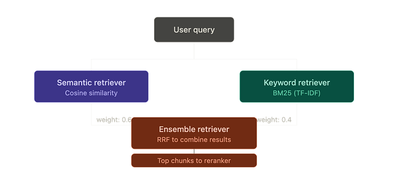
To combine semantic and keyword search, you use an ensemble retriever. It runs both retrievers in parallel and merges their results using RRF, which we covered in the previous section.
What makes the ensemble retriever flexible is weighting. You can control how much you want to lean toward semantic results versus keyword results. A knowledge base full of technical documentation with specific product codes might warrant a higher keyword weight. A conversational FAQ might lean more semantic. The weights feed directly into the RRF scoring as numerators, so tuning them shifts which retriever has more influence over the final ranking.
In production
A production-grade retrieval setup combines everything from the last two sections: multiple query variants, run across both semantic and keyword retrievers, with RRF merging the results.
Even then, you’re often left with more chunks than you want to pass to the LLM. Running multi-query hybrid search can surface 20 to 30 candidate chunks. Passing all of them increases cost, latency, and the risk of noisy context degrading the answer quality.
This is where reranking comes in: a final filtering step that scores the merged candidates more carefully and cuts the list down to the top 5 or top 10 before anything reaches the LLM. We’ll cover that in the next section.
9. Reranking
After hybrid search and RRF, you might still have 20 to 30 candidate chunks. Passing all of them to the LLM would bloat the context window, increase cost and latency, and reintroduce the exact noise problem RAG was designed to solve. In production you want to pass the top 5 to 10 chunks, no more.
But how do you decide which 5 to 10 are the best ones? The similarity scores from vector search are good approximations, not precise relevance scores. This is where a reranker comes in.
A reranker is a model that sits between the retriever and the LLM. It takes every candidate chunk, scores it carefully against the query, and reorders the list so you can confidently cut it at the top.
The two stage process
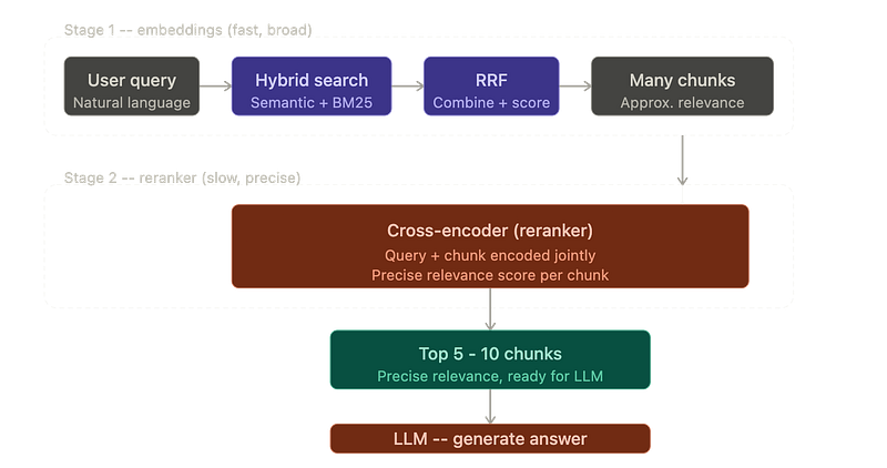
It helps to think of the full retrieval pipeline as two distinct stages with different jobs:
Stage 1, embeddings: fast and broad. You cast a wide net using vector similarity. This is intentionally an approximation: you’re finding chunks that are roughly in the right direction, not necessarily the most relevant ones. Speed is the priority here.
Stage 2, reranker: slow and precise. For each chunk returned in stage 1, the reranker takes the query and the chunk together, encodes them jointly, and produces a precise relevance score. This is repeated for every candidate, then the list is reordered by these scores and trimmed.
The two-stage design is deliberate. Running a precise reranker over your entire vector DB on every query would be too slow. Running only fast vector search gives you speed but imprecision. Together, you get the best of both.
Bi-encoder vs cross-encoder
Understanding this distinction explains why reranking is more accurate than embedding alone.
An embedding model is a bi-encoder. It encodes the query into a vector and each chunk into a vector separately, then compares them after the fact. It’s fast because the chunk vectors can be precomputed and stored. But encoding them separately means the model never gets to see how the query and chunk interact with each other. It’s comparing two things in isolation.
A reranker is a cross-encoder. It takes the query and the chunk concatenated together as a single input and encodes them jointly. Because the model sees both at the same time, it can capture much richer signals: does the chunk directly answer the question, or just share some keywords? Is the relevance explicit or just implied? This joint encoding produces a relevance score that’s meaningfully more accurate than cosine similarity.
The tradeoff is that cross-encoders can’t precompute anything. Every query requires a fresh pass over every candidate chunk, which is why you use the bi-encoder to filter down to a manageable set first. Cohere’s reranker is one of the most widely used options in production.
Where to go from here?
This post covered the full architecture of a RAG system, from the ingestion pipeline and chunking strategies to hybrid search, RRF, and reranking. By now you should have a solid mental model of how a production RAG system is actually built.
But building the pipeline is only half the story. Once it’s running, a new set of questions takes over:
What actually breaks in production, and how do you diagnose it? How do you ensure reliability when your knowledge base changes? What does hallucination look like in a RAG system specifically, and how do you reduce it? How do you evaluate whether your RAG system is good, not just working?
These are the questions that separate a RAG proof-of-concept from a production system you can trust.
I’ll be covering each of them in the next part of this series.